
Basic NONMEM Workshop Instructions
Objectives
Objectives
- To provide practical experience of performing population pharmacokinetic analysis using NONMEM.
- To learn how to construct models describing:
- residual error
- structure and variability
- covariate effects
Installation
Installation
A zip archive executable file nm72p.exe is provided for installation of NONMEM and related files for the HandsOn sessions.
If you have write access to your C: drive then open the nm72p.exe file and extract the files to \nm72P (the default location).
You may also extract the files to a USB drive but NONMEM will run more slowly.
Session 1 - Introduction to NONMEM and Residual Error Models
Session 1 - Introduction to NONMEM and Residual Error Models
A data set is provided (warfpk.csv) which describes the pharmacokinetics of warfarin in healthy subjects. A dose of 1 mg/kg was given orally and warfarin concentrations measured using a non-stereoselective assay including both bound and unbound warfarin.
Note: All files should be loaded from and saved to your \nm72P\My Pharmacometrics\Pharmacometrics Data\Basic\Session 1 - interpret output folder for this session.
- Use Windows Explorer to explore the My Pharmacometrics\Pharmacometrics Data\Basic\Session 1 - interpret output folder.
- Open the warfpk.csv file using Excel and examine its structure and contents.
- Open the warf_addRUV.ctl file and look at the NM-TRAN control stream code.
- Open a Wings for NONMEM command line window by double clicking on the My Pharmacometrics\Pharmacometrics Programs\NONMEM shortcut.
- Change directory to Session 1 by typing "cd S" then press the Tab key until you see Session 1 appear then press Enter to change to this directory
cd "Session 1 - interpret output"
- Start a NONMEM run using the warf_addRUV.ctl NM-TRAN control stream with:
nmgo warf_addRUV
- When the run is finished the results will be shown in a table format extracted from the NONMEM output listing.
- Repeat steps 2 to 4 with the warf_propRUV and warf_combRUV control streams.
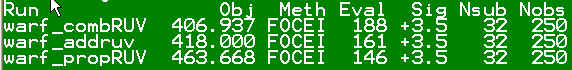
- Look at a summary of the run results using the nmobj command.
nmobj
- Create a model building table file using the nmmbt command.
nmmbt
- Open the nmmbt.txt file with Excel and compare the parameter estimates from each run.
Session 2 - Building Structural and Variability Models
Session 2 - Building Structural and Variability Models
This session uses the same warfarin data used for Session 1.
Note: All files should be loaded from and saved to your \nm72P\My Pharmacometrics\Pharmacometrics Data\Basic\Session 2 - build structural model folder for this session.
- Use Windows Explorer to explore the My Pharmacometrics\Pharmacometrics Data\Basic\Session 2 - build structural model folder.
- Open the warf_addRUV.ctl file and look at the NM-TRAN control stream code.
- Change directory to Session 2 by typing "cd S" then press the Tab key until you see Session 2 appear then press Enter to change to this directory
cd "Session 2 - build structural model"
- Open a Wings for NONMEM command line window by double clicking on the My Pharmacometrics\Pharmacometrics Programs\NONMEM shortcut.
- Start a NONMEM run using the warf_combRUV_lag.ctl NM-TRAN control stream with:
nmgo warf_combRUV_lag
- When the run is finished the results will be shown in a table format extracted from the NONMEM output listing.
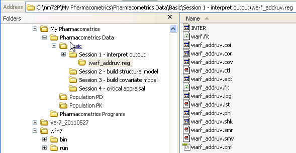
- Locate the warf_addRUV.fit file using Windows Explorer.
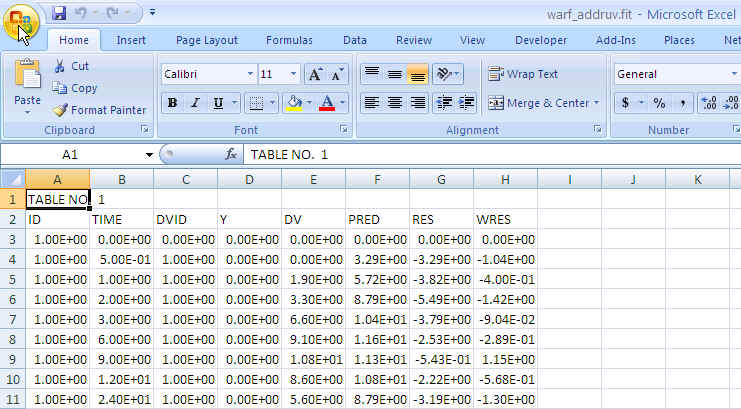
- Open the warf_addRUV.fit file using Excel.
- Click on Finish when the Text Import wizard opens
- Remove the scientific notation by Right click on upper left corner of the spreadsheet (just to the left of the column heading A), click on Format cells..., select General.
- Delete the first row ("TABLE NO 1").
- Create a plot of PRED vs RES. Highlight the PRED and RES columns then click Insert, then Scatter, then choose Scatter with only markers.
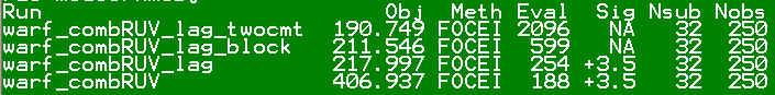
- Repeat steps 2 to 4 with the warf_combRUV_lag_block and warf_combRUV_lag_twocmt control streams.
- Run the warf_combRUV model which you used in Session 1 so you can compare the results with model used in Session 2.
- Look at a summary of the run results using the nmobj command.
nmobj
- Create a model building table file using the nmmbt command.
nmmbt
- Open the nmmbt.txt file with Excel and compare the parameter estimates from each run.
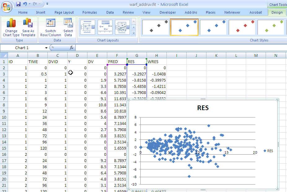
Excel warf_ruv PRED vs RES: No obvious trend
Session 3 - Building Covariate Models
Session 3 - Building Covariate Models
This session uses the same warfarin data used for Session 1.
Note: All files should be loaded from and saved to your \nm72P\My Pharmacometrics\Pharmacometrics Data\Basic\Session 3 - build covariate model folder for this session.
- Use Windows Explorer to explore the My Pharmacometrics\Pharmacometrics Data\Basic\Session 3 - build covariate model folder.
- Open the warf_base.ctl file and look at the NM-TRAN control stream code. Confirm that this is similar to the warf_combRUV_lag.ctl with the addition of ETA(1) and ETA(2) to the $TABLE record
- Open a Wings for NONMEM command line window by double clicking on the My Pharmacometrics\Pharmacometrics Programs\NONMEM shortcut.
- Change directory to Session 3 by typing "cd S" then press the Tab key until you see Session 3 appear then press Enter to change to this directory.
cd "Session 3 - build covariate model"
- Start a NONMEM run using the warf_base.ctl NM-TRAN control stream with:
nmgo warf_base
- When the run is finished the results will be shown in a table format extracted from the NONMEM output listing.
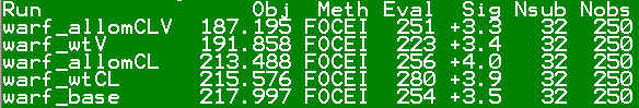
- Repeat steps 2 to 4 with the warf_wtV, warf_wtCL,warf_allomCL and warf_allomCLV control streams.
- Look at a summary of the run results using the nmobj command.
nmobj
-
Note that the order you add the covariates changes the significance of the covariates. See here that adding allometric WT on CL was barely significant over the base model (drop in OFV by 4.5 points). But adding allometric WT on CL after adding WT on V was highly significant (drop in OFV of 30.8 points).
- Create a model building table file using the nmmbt command.
nmmbt
- Open the nmmbt.txt file with Excel and compare the parameter estimates from each run.
Visual Evaluation Methods
Visual Evaluation Methods
- Residual plots created with Excel.
- Visual Predictive Checks using WFN
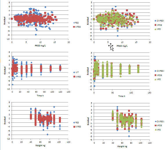
Excel warf_addruv Residuals: +ve at low and -ve at high weight ?
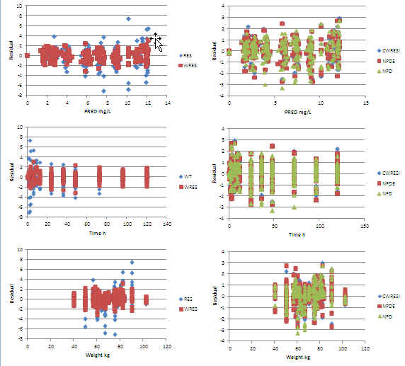
Excel warf_allomCLV Residuals: No trends
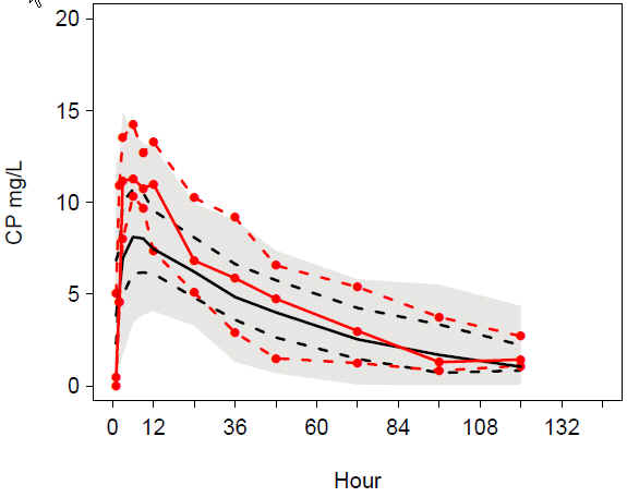
VPC addruv TIME female: Underprediction around peak
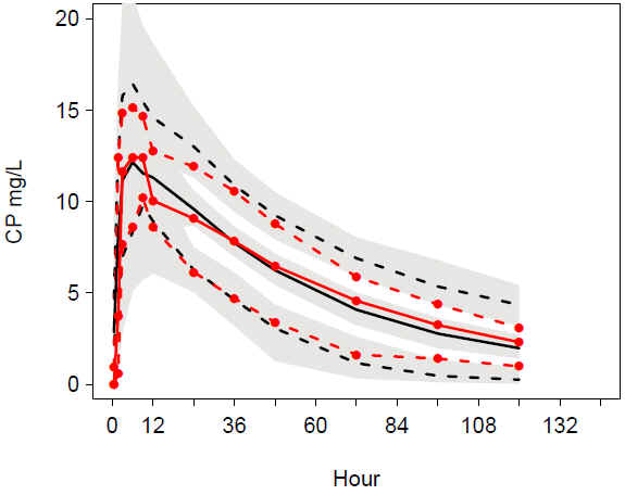
VPC addruv TIME male: Good match of observations and predictions
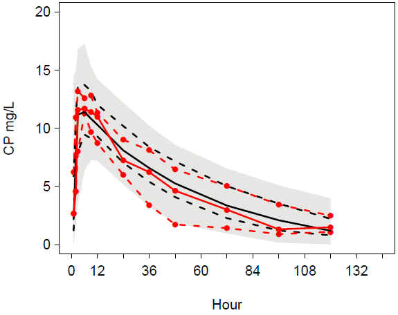
VPC allomCLV TIME female:Better match of observations and predictions
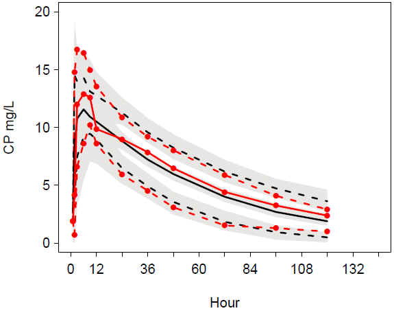
VPC allomCLV TIME male: Good match of observations and predictions
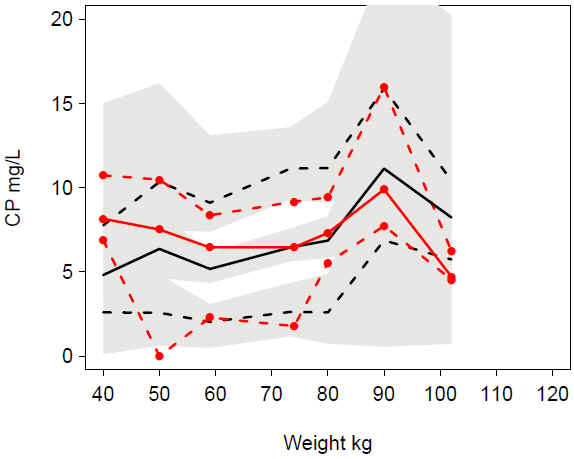
VPC warf_addruv WT: Undeprediction at low WT, overprediction at high WT
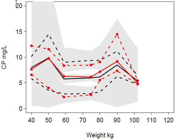
VPC warf_alloCLV WT: Good match of observations and predictions